Introduction
This article examines the monthly mean atmospheric carbon dioxide concentrations recorded at the National Oceanic and Atmospheric Administration (NOAA), Mauna Loa Observatory in Hawaii. The measurements are reported as mole fractions, expressed in parts per million (ppm). In practical terms, a concentration of 400 ppm means that approximately 400 out of every one million molecules of air are Carbon Dioxide (CO2) molecules.
The dataset contains monthly observations beginning in 1958, as documented by NOAA.
The variable average represents the observed monthly mean CO2 concentration and serves
as the principal time series used throughout the analysis.
The objective is to demonstrate the full workflow of a time-series analysis by investigating the key statistical properties of the monthly CO2 series. The analysis begins by exploring the observed series and assessing its underlying structure. It then examines stationarity and applies the necessary tests to prepare the series for modelling, followed by the identification and selection of an appropriate time-series model. The selected model is subsequently evaluated through residual diagnostics to assess whether it adequately captures the temporal structure of the data.
Once the model has been validated, it is used to produce a multi-month forecast of atmospheric CO2 concentrations, together with corresponding confidence intervals. Forecast performance is then assessed using a chronological out-of-sample holdout set, allowing the predicted values to be compared directly with the observed CO2 concentrations. Finally, the forecasting performance of the selected time-series model is compared with that of Triple Exponential Smoothing, providing an additional benchmark for evaluating its predictive performance.
- Time-series analysis is a broad subject, with entire courses and textbooks devoted to its theory and mathematical foundations. This article focuses on the practical workflow, modelling decisions, and interpretation of results, rather than attempting to cover every formulation, derivation, or proof in detail.
- The analysis is implemented in Python; however, the code itself is not explained in this article. Basic to intermediate programming knowledge is assumed for readers who wish to reproduce the analysis, modify the code, or run the examples themselves.
- For those interested in the technical implementation, a fully documented Jupyter Notebook is provided in this GitHub repository, containing all code, outputs, figures, and additional detailed Markdown explanations supporting the analysis.
1. Exploring the Raw CO2 Series
Before applying any transformations or fitting models, we first load and clean the data, structure the observations as a monthly time series, and perform a chronological train-holdout split. With the data prepared and the holdout period reserved for later out-of-sample validation, we can now examine the raw CO2 series to identify its main temporal characteristics.
As shown in Figure 1, the raw monthly CO2 time series exhibits two dominant characteristics: a pronounced long-term upward trend and a clear recurring annual seasonal cycle. The concentration rises from approximately 315 ppm in the late 1950s to more than 420 ppm in recent years, while simultaneously exhibiting regular within-year fluctuations.
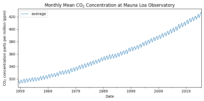
Figure 1: Monthly atmospheric CO2 concentration recorded at Mauna Loa.
The combination of a changing long-term level and recurring seasonal behaviour means that the statistical properties of the raw series are not constant through time. This is an important indication that the raw CO2 series is non-stationary. These characteristics motivate the use of time-series methods capable of handling both non-seasonal and seasonal dynamics, such as Triple Exponential Smoothing and SARIMA models.
1.1 Stationarity of the Raw CO2 Series
The raw CO2 series shows clear signs of strong temporal dependence, but visual patterns alone are not sufficient to establish stationarity. We therefore examine its autocorrelation structure using the Autocorrelation Function (ACF) and Partial Autocorrelation Function (PACF), followed by the Augmented Dickey-Fuller (ADF) test and Kwiatkowski-Phillips-Schmidt-Shin (KPSS) tests for formal statistical confirmation.
(a) ACF and PACF of the Raw CO2 Series
The ACF measures the correlation between observations at different time lags, while the PACF measures the correlation at a given lag after accounting for the effects of shorter lags. Because the data are monthly, particular attention is given to lag 12 and its multiples, which correspond to annual seasonal relationships.
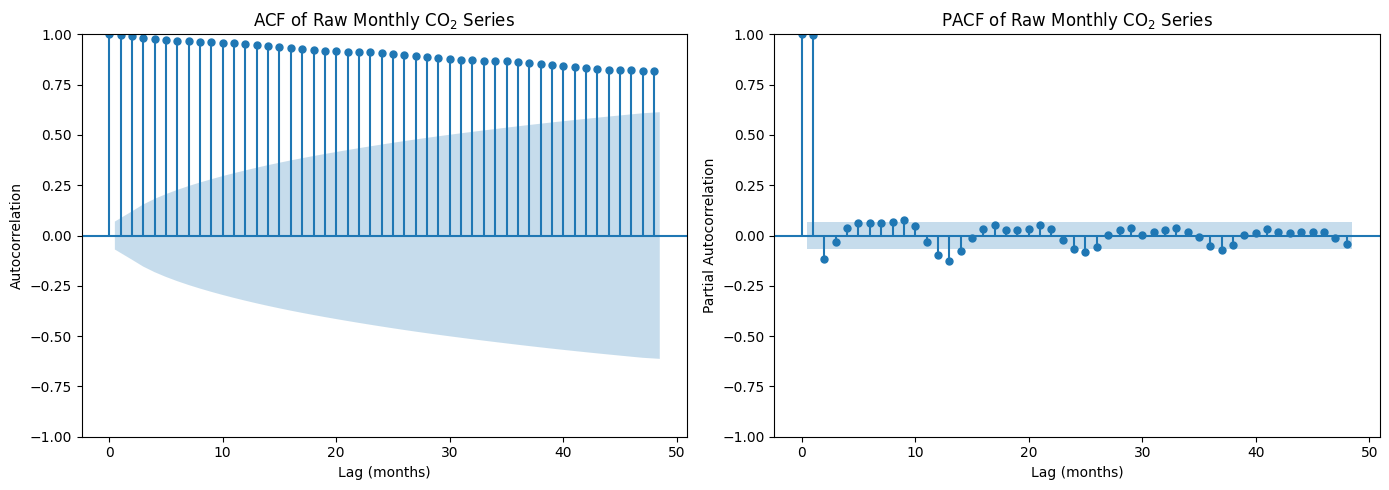
Figure 2: ACF and PACF of the raw monthly CO2 series.
Figure 2: shows that the ACF remains strongly positive across many lags and decays slowly. Such behaviour is characteristic of a highly persistent, non-stationary series with a strong underlying trend. Taken together, the ACF and PACF provide visual evidence of strong temporal dependence, trend, and seasonality in the raw series.
(b) Formal Stationarity Tests: ADF and KPSS
While the ACF and PACF provide useful visual evidence, stationarity is assessed more formally using two complementary tests: the ADF test and the KPSS test. The ADF and KPSS tests approach stationarity from opposite directions: for the ADF test, a small p-value provides evidence against the null hypothesis of a unit root and supports stationarity, whereas for the KPSS test, a small p-value leads to rejection of the null hypothesis of stationarity and supports non-stationarity. The formal null and alternative hypotheses, together with the corresponding decision rules, are detailed in the accompanying notebook.
The test results, which were reproduced in the accompanying notebook, provide consistent evidence that the raw CO2 series is non-stationary.
The ADF test produces a p-value: p = 1.0000, which is substantially greater than 0.05; we therefore fail to reject the null hypothesis of a unit root.
The KPSS test reported p-value: p = 0.0100, which is below 0.05; consequently, the null hypothesis of stationarity is rejected.
Furthermore, the test statistics reinforce these conclusions: the ADF Test statistic: ADF = 6.2373 lies well above all its reported critical values, while the KPSS Test statistic: KPSS = 4.2289 lies well above all its
critical values. Taken together, both tests point to the same conclusion—the raw CO2 series is non-stationary. This is consistent with the pronounced upward
trend and recurring annual seasonality observed in the time plot and ACF/PACF analysis, indicating that transformation is required before proceeding to time-series model fitting.
2. Differencing the CO2 Series
Differencing is one of the principal tools used to remove non-stationarity from a time series. Two common transformations are regular differencing and log differencing. In our case, regular first differencing measures the absolute month-to-month change:
\[ \Delta CO_{2,t} = CO_{2,t} - CO_{2,t-1}. \]In contrast, log differencing would measure proportional change:
Since CO2 is measured in ppm and the objective is to model changes in the physical concentration rather than percentage growth, absolute (regular) differencing is used here. Log differencing would be more natural if the principal interest were relative or percentage changes.
- The distinction between Regular differencing and Log differencing is particularly important in financial time series, where log differences are commonly interpreted as log returns. They describe relative changes in an asset's value rather than changes in its price in absolute units.
- We have seen that Log differencing is defined as; \( \Delta \log(Y_t) = \log(Y_t)-\log(Y_{t-1}), \)
- Using the logarithm rule, this can equivalently be written as; \( \Delta \log(Y_t) = \log\left(\frac{Y_t}{Y_{t-1}}\right), \)
- Since: \[ \frac{Y_t}{Y_{t-1}} = 1+\frac{Y_t-Y_{t-1}}{Y_{t-1}}, \] log differencing can also be expressed as; \( \Delta \log(Y_t) = \log\left( 1+\frac{Y_t-Y_{t-1}}{Y_{t-1}} \right). \) It therefore measures a logarithmic proportional change.
- For relatively small proportional changes, Taylor expansion of \(\log(1+x)\) around \(x=0\), \[ \log(1+x) = x-\frac{x^2}{2}+\frac{x^3}{3}-\cdots, \] shows that the higher-order terms become negligible, giving the approximation; \( \log(1+x)\approx x. \) Therefore; \[ \Delta\log(Y_t) \approx \frac{Y_t-Y_{t-1}}{Y_{t-1}}, \] meaning that log differences can be interpreted approximately as proportional changes or growth rates.
2.1 Regular First Differencing
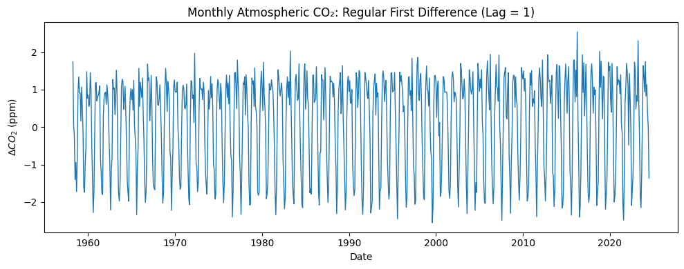
Figure 3: Monthly first differences of atmospheric CO2 concentration.
From Figure 3 we see that regular first differencing substantially removes the long-term upward trend. The transformed series fluctuates around a comparatively stable level rather than continuing to rise over time. However, a pronounced seasonal oscillation remains. This demonstrates an important distinction: regular differencing can remove much of the non-seasonal trend without necessarily removing the annual seasonal component.
2.2 ACF and PACF After Regular Differencing
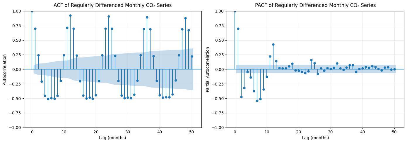
Figure 4: ACF and PACF of the regularly differenced CO2 series.
The ACF shows pronounced positive autocorrelation around the 12-month lag, together with additional peaks around 24, 36, and 48 months. This repeating structure is characteristic of an annual seasonal cycle. The PACF also shows significant dependence at short and seasonal lags. Thus, regular differencing has addressed much of the long-term trend but has not eliminated the annual seasonal structure. These observations motivate further investigation of seasonal differencing with a period of 12 months.
2.3 Monthly Distribution of the Regularly Differenced Series
The remaining seasonal structure can be examined more directly by grouping the first differences according to calendar month. Because the series has been differenced, a positive value means that CO2 increased relative to the preceding month, while a negative value means that the concentration decreased:
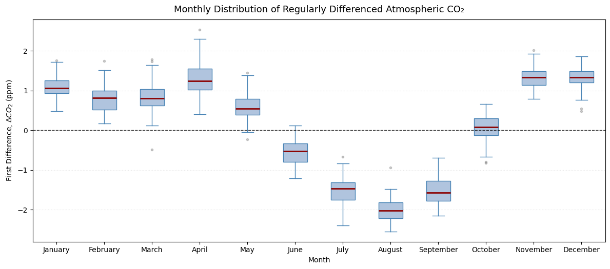
Figure 5: Distribution of monthly CO2 changes by calendar month.
Figure 5 shows that the monthly distributions vary systematically across the calendar year. In particular, July, August, and September show substantially more negative first differences. This means that atmospheric CO2 concentrations decreases during this part of the year.
What Causes the Monthly Seasonal Pattern?
The observed seasonal behaviour is physically consistent with the dominant influence of the terrestrial biosphere on atmospheric CO2. The seasonal CO2 cycle is particularly strong because a large proportion of the Earth's land area and vegetation is located in the Northern Hemisphere. During Northern Hemisphere spring and summer, increased photosynthetic activity removes CO2 from the atmosphere, while during autumn and winter, reduced photosynthesis and continued respiration & decomposition return more CO2 to the atmosphere.
Additionally, during the Northern Hemisphere winter, when photosynthetic CO2 uptake is substantially reduced, energy demand for heating generally increases. The associated combustion of fossil fuels for heating and electricity generation, together with continued transportation and other human activities, adds more CO2 to the atmosphere during a period when natural terrestrial uptake is relatively weak. The combination of these factors produces a recurring annual oscillation and upward trend in atmospheric CO2 concentrations.
Why Does the Southern Hemisphere Not Cancel the Northern Hemisphere Cycle?
Although the Southern Hemisphere experiences its growing season while the Northern Hemisphere is in winter, its influence is considerably weaker. The key reason is the strong asymmetry in land and vegetation distribution between the two hemispheres. The Northern Hemisphere contains substantially more land and terrestrial vegetation, whereas the Southern Hemisphere is dominated by oceans.
This means that the seasonal uptake and release of CO2 by Northern Hemisphere terrestrial ecosystems is much larger than the corresponding seasonal cycle in the Southern Hemisphere. The Southern Hemisphere therefore partially offsets the Northern Hemisphere signal, but not enough to cancel it. Therefore, the resulting global atmospheric CO2 record retains a pronounced annual cycle dominated by the Northern Hemisphere biosphere.
2.4 Stationarity Tests After Regular First Differencing
The ADF and KPSS tests are repeated after applying regular first differencing to determine whether the transformed series now satisfies the stationarity requirement.
| Test | Statistic | p-value | Lags Used | Interpretation |
|---|---|---|---|---|
| ADF | -11.2895 | 0.0000 | 12 | Reject unit root; evidence of stationarity |
| KPSS | 0.0456 | 0.1000 | 30 | Fail to reject stationarity |
The ADF statistic of -11.2895 is substantially more negative than
all reported critical values. In particular, it is well below the 1% critical value
of -3.4389, as well as the 5% and 10% critical values of
-2.8653 and -2.5688, respectively. The reported
p-value is 0.0000 to the numerical precision of the test output,
indicating that the actual p-value is less than 0.001. Therefore,
the null hypothesis of a unit root is rejected, providing strong evidence that the
regularly first-differenced series is stationary.
The KPSS statistic of 0.0456 is far below the 10% critical value of
0.3470. It is also below the 5%, 2.5%, and 1% critical values of
0.4630, 0.5740, and 0.7390,
respectively. The reported p-value is 0.1000
(interpolation warning indicates that the actual p-value is even greater than 0.10).
This results suggest that the null hypothesis of stationarity is therefore not rejected.
Taken together, the ADF and KPSS tests provide consistent evidence that the series becomes stationary after one regular difference. These results therefore support a regular differencing order of: \(\boxed{d=1}\). Importantly, this value provides the regular differencing component for subsequent SARIMA model development. However, the complete model must still be evaluated using information criteria and residual diagnostics.
Since regular first differencing achieves stationarity, the discussion in this article does not proceed further with combined differencing (regular first differencing together with seasonal differencing). However, the accompanying notebook explores this additional step in greater detail. Readers interested in exploring the combined differencing approach are encouraged to consult the accompanying Jupyter Notebook, where detailed analysis is documented in the Markdown sections.
3. SARIMA Model Specification and Selection
The preceding analysis established that the CO2 series contains a strong trend and annual seasonal structure. Regular and seasonal differencing produced a stationary transformed series, supported by both the ADF and KPSS tests. The next step is to model the original CO2 series using a Seasonal Autoregressive Integrated Moving Average (SARIMA) model. A general SARIMA model is written as:
\[ \mathrm{SARIMA}(p,d,q)\times(P,D,Q)_s \]Here, \(p\) and \(q\) describe the non-seasonal Autoregressive (AR) and Moving-average (MA) components, while \(P\) and \(Q\) describe their seasonal counterparts. The parameters \(d\) and \(D\) specify regular and seasonal differencing, and \(s\) is the seasonal period. Model selection considers several complementary criteria:
- AIC (Akaike Information Criterion): balances model fit against model complexity, with lower values indicating a preferred model.
- BIC (Bayesian Information Criterion): also balances model fit and complexity, but applies a stronger penalty for additional parameters than AIC.
- Residual diagnostics: the residuals should contain little or no remaining temporal structure, indicating that the model has adequately captured the systematic patterns in the data.
- Parameter significance: estimated model parameters should generally be statistically meaningful and contribute to explaining the observed dynamics.
- Residual variance and stability: residual variability should remain reasonably stable over time, with no strong evidence of changing variance or other systematic instability.
3.1 Selected SARIMA Model
Several models were fitted to the raw CO2 concentration series. Following a comprehensive comparison and evaluation of the candidate models, the model selected was:
\[ \boxed{ \mathrm{SARIMA}(0,1,2)\times(8,0,0)_{12} } \]The final specification differs from the initially proposed model. It retains regular differencing \(d\), but does not use seasonal differencing \(D\). Instead, annual dependence is represented through eight seasonal autoregressive terms corresponding to lags: \(12,\ 24,\ 36,\ 48,\ 60,\ 72,\ 84,\ 96.\) While the non-seasonal component is an \(MA(2)\) process.
The selected model produced a log-likelihood of -193.828, with
an AIC of 409.656, a BIC of 459.718, and an HQIC of 429.008.
When selecting the best model, these information criteria were considered alongside parameter significance and residual behaviour, rather than being used in isolation.
A detailed discussion of the remaining model output—including the non-seasonal MA component, the seasonal autoregressive structure,
and the analysis of the estimated innovation variance—is provided in the accompanying notebook.
Overall, the selected SARIMA model represented the CO2 dynamics through regular differencing, short-term moving-average effects, and a rich annual autoregressive structure.
- A simple way to assess whether a time-series model coefficient \(\hat{\beta}\) is statistically significant is to compare it with approximately two standard errors. If the coefficient itself lies outside the range: \[ \left[-2SE(\hat{\beta}),\,+2SE(\hat{\beta})\right], \] it is approximately significant at the 5% level. Equivalently, if the resulting interval does not contain zero, the coefficient is also approximately significant at the 5% level.
- This rule is a convenient approximation to the usual 95% confidence interval, \[ \hat{\beta} \pm 1.96\,SE(\hat{\beta}), \] derived from the normal approximation. Thus, the familiar ±2 standard errors rule is simply a rounded \(1.96\).
4. Residual Diagnostics and Model Adequacy
Once the model had been fitted, the next question was whether it had actually captured the systematic structure in the data. This was assessed through its residuals, which represent the portion of the observations not explained by the model. Ideally, the residuals should behave approximately like white noise: meaning they should contain little systematic autocorrelation, have reasonably stable variance, and preferably be approximately normally distributed.
Several diagnostic checks are normally used to evaluate whether the selected model has adequately captured the systematic structure and patterns in the data:
- White-Noise Check: Ljung-Box Test: This test examines whether the residuals contain significant autocorrelation across a set of lags.
- Normality of the Residuals: Residual normality is assessed using the Jarque-Bera and D'Agostino-Pearson tests, together with a histogram and Normal Q-Q plot.
- Residual Variance and Distribution: The residual time plot and histogram are also examined for; changing variance over time, extreme outliers, strong skewness and unusually heavy tails.
4.1 Ljung-Box Test: Checking for Remaining Autocorrelation
Because the CO2 series exhibits a strong annual cycle, the Ljung-Box test was evaluated at several seasonal horizons, including \(12,\ 24,\ 36,\ 48,\ 60,\) and \(72\) months, thereby covering multiple annual cycles. A more detailed discussion of the Ljung-Box test—including its null and alternative hypotheses, decision rule, and interpretation—is provided in the accompanying notebook.
Ideally, for a well-specified time-series model, we expect the Ljung-Box test to produce a p-value greater than 0.05. In this case, we therefore fail to reject \(H_0\), which states that there is no statistically significant autocorrelation in the residuals up to the specified lag.
The residual analysis of our series provides strong evidence that the selected model has successfully removed the major serial dependence present in the original series. As shown in Table 2, every p-value is substantially greater than the 0.05 significance level. In particular, the results remain non-significant well beyond the annual seasonal period of 12 months, extending to 72 months. Meaning we therefore fail to reject the null hypothesis at every tested horizon, providing no evidence of statistically significant residual autocorrelation.
| Lag | Q-statistic | p-value |
|---|---|---|
| 12 | 3.006 | 0.9955 |
| 24 | 5.689 | 0.99996 |
| 36 | 8.208 | 1.0000 |
| 48 | 8.841 | 1.0000 |
| 60 | 9.043 | 1.0000 |
| 72 | 10.090 | 1.0000 |
This represents a strong piece of evidence in favour of the selected model. The rich seasonal AR structure appears to have captured the annual dependence sufficiently well that the remaining residuals contain no detectable systematic autocorrelation.
It is important to distinguish the Ljung-Box statistic, which is normally shown in the SARIMAX model
summary, from the broader diagnostic analysis. The model summary reports a lag-1
diagnostic, whereas the analysis here examines substantially longer horizons.
4.2 Residual Normality
Residual normality is assessed using the Jarque-Bera and D'Agostino-Pearson tests, together with the residual histogram and Normal Q-Q plot. For normally distributed residuals, we would expect approximately: \({Skewness}\approx0,\) and \({Kurtosis}\approx3.\) The Jarque-Bera test evaluates whether the distribution is compatible with normality based primarily on skewness and kurtosis. A p-value below 0.05 indicates statistically significant departure from normality.
For our model, the Jarque-Bera test yields \({JB = 18{,}427{,}159.13,\hspace{0.3em}p < 0.001}\), while the D'Agostino-Pearson test yields \(K^2 = 2064.01,\hspace{0.3em}p < 0.001\). Both tests strongly reject the null hypothesis of normally distributed residuals. The corresponding skewness and kurtosis estimates are \({Skewness} = 26.80,\) and \({Kurtosis} = 745.98\), indicating substantial departure from normality. These values are extremely large. However, the residual summary analysis indicates that the result is driven by a very small number of extreme observations. A more detailed account of this analysis is provided in the accompanying notebook.
4.3 Residual Variance and Distribution
The residual time series plot, histogram, and Q-Q plot are also examined for systematic trends, changing variance, extreme observations, skewness, and unusually heavy tails. These diagnostic plots indicate that the principal departure from normality occurs in the tails, while the central bulk of the observations is considerably more concentrated. This reinforces the interpretation that extreme residuals are concentrated in a small number of historical observations rather than representing the typical behaviour of the process.
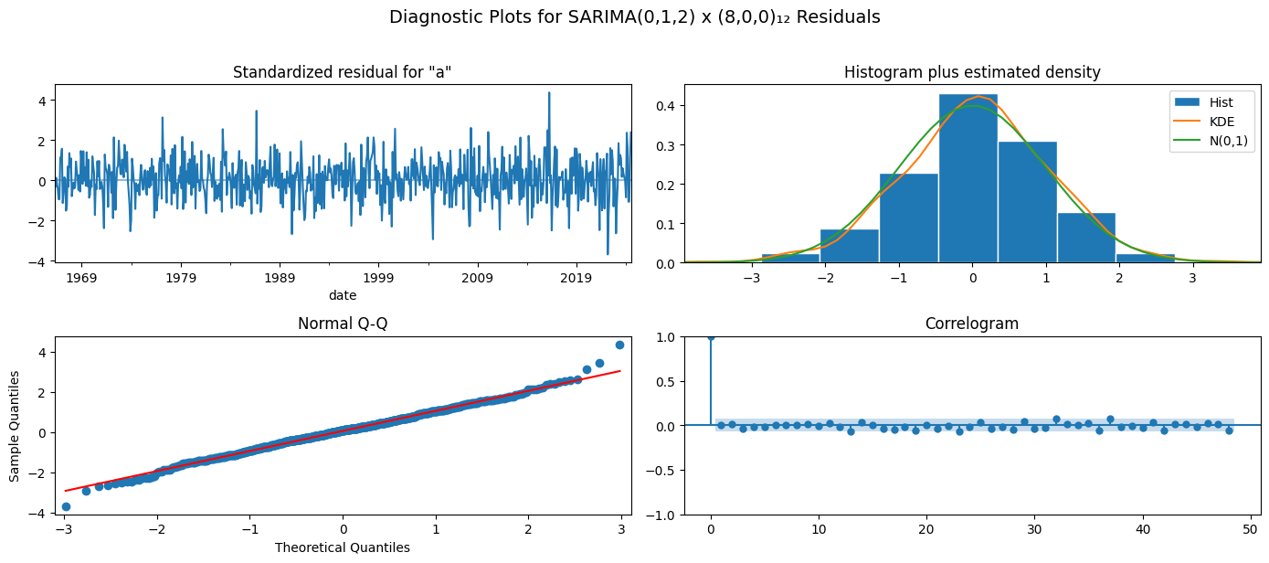
Figure 6: Residual diagnostic plots for the selected SARIMA model.
4.4 Residual ACF and PACF
The residual ACF and PACF were examined through a lag of 60 months using 95% confidence bounds. Figure 9 shows that none of the coefficients exhibits a clear spike outside the corresponding confidence limits. In particular, there are no obvious significant spikes at the seasonal lags of 12, 24, 36, 48, or 60 months. This is consistent with the Ljung-Box results and provides visual evidence that little systematic temporal dependence remains.
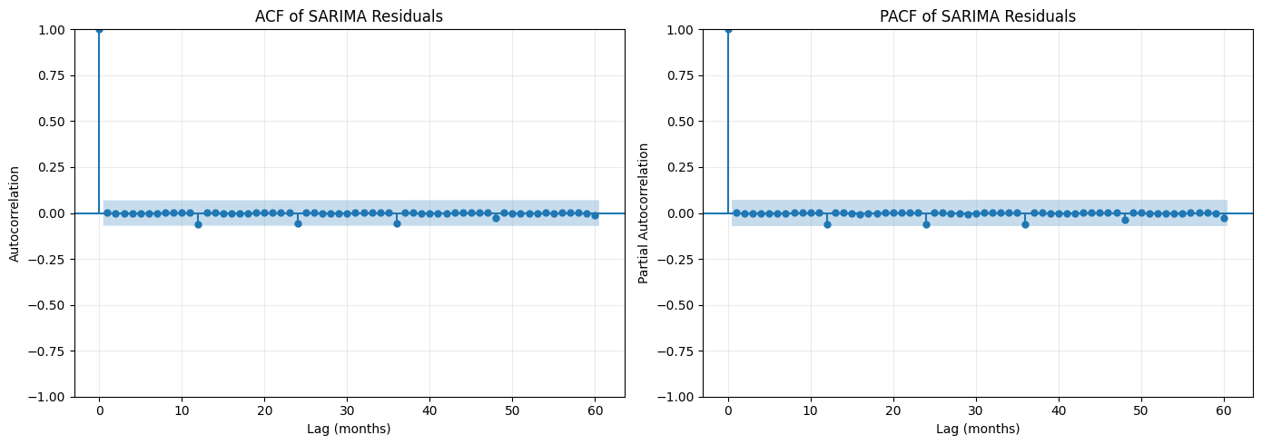
Figure 9: Residual ACF and PACF through 60 months.
4.5 Overall Model Adequacy
The residual diagnostics therefore provide a mixed but informative assessment: The Ljung-Box results are highly satisfactory: all tested horizons produce p-values far above 0.05, indicating no evidence of remaining serial correlation. The normality tests strongly reject Gaussian residuals, but the extreme skewness and kurtosis are largely driven by a small number of unusually large observations, particularly the March 1958 residual.
- The Ljung-Box results are highly satisfactory: all tested horizons produce p-values far above 0.05, indicating no evidence of remaining serial correlation.
- The normality tests strongly reject Gaussian residuals, but the extreme skewness and kurtosis are largely driven by a small number of unusually large observations, particularly the March 1958 residual.
Approximate normality is desirable because the standard Gaussian SARIMA framework commonly assumes normally distributed innovations, implying that the model errors should be approximately Gaussian with constant variance. However, exact normality is not essential for assessing the model's dynamic adequacy. A more fundamental requirement is that the residuals contain no substantial remaining temporal dependence.
The Ljung-Box results and ACF/PACF plots support this condition, indicating that the residuals behave approximately as white noise with respect to temporal dependence. Thus, there is no evidence of substantial remaining serial dependence, suggesting that the model adequately captures the underlying temporal structure of CO2 concentration series.
5. Forecasting the CO2 Series
After selecting and validating the SARIMA model, the next objective is to forecast future atmospheric CO2 concentrations. Forecasts are generated on the original concentration scale so that the results can be interpreted directly in ppm. Additionally, the forecast horizon is 24 months, allowing the model's ability to reproduce both the short-term evolution and the annual seasonal pattern to be examined over more than one complete seasonal cycle.
5.1 Forecast on the Original CO2 Scale
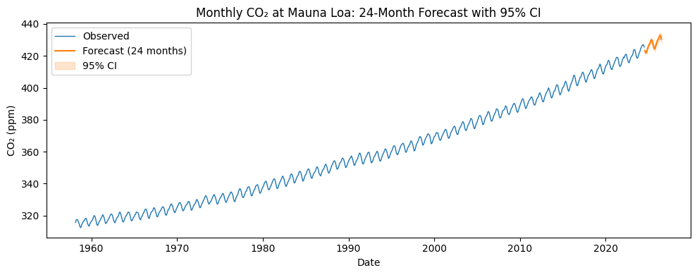
Figure 8: SARIMA forecast with 95% confidence intervals on the original CO2 scale.
Figure 8 shows that the forecast continues the overall upward trajectory of the historical CO2 series while retaining its pronounced annual seasonal fluctuations. This is important because the model is not merely extrapolating a simple linear trend. The seasonal autoregressive structure allows information from previous annual cycles to contribute to future predictions. The 95% confidence interval becomes wider as the forecast horizon increases. This is expected in multi-step forecasting because uncertainty accumulates as predictions extend further beyond the final observed value.
These intervals should nevertheless be interpreted with some caution because the residual analysis found substantial departures from Gaussianity caused by extreme historical observations. Standard SARIMAX confidence intervals rely on the model's innovation assumptions and may therefore not fully capture the probability of unusually large future deviations.
5.2 Out-of-Sample Forecast Validation
A much stronger test of forecasting performance is obtained by comparing predictions against observations that were deliberately withheld during model estimation. The model is therefore evaluated against the chronological holdout period. Because these observations were not used to estimate the model parameters, they provide genuinely out-of-sample evidence of predictive performance.
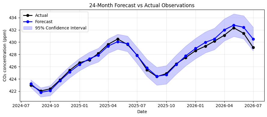
Figure 9: SARIMA forecast compared with the unseen holdout observations.
As seen in Figure 9 the forecast follows the actual CO2 observations remarkably closely across the validation period. It reproduces both the overall upward movement and the recurring seasonal fluctuations. This type of chronological validation is considerably more informative than judging model performance solely from an in-sample fit. A model that performs well on data it has already seen may still perform poorly when asked to predict the future. In this case, the close correspondence between forecasts and observations suggests that the model has learned meaningful temporal structure rather than simply fitting historical noise.
The actual observations also remain within the corresponding 95% confidence bands throughout the validation period shown. This provides encouraging evidence that the model's uncertainty estimates are reasonably consistent with the observed variation, although it does not by itself establish perfect statistical calibration.
6. Comparison with Triple Exponential Smoothing
A SARIMA model is not the only way to forecast a series with trend and seasonality. To provide an alternative benchmark, the forecasting performance is compared with Triple Exponential Smoothing, also known as the Holt-Winters method. Triple Exponential Smoothing explicitly models three components: \(\boxed{\text{Level}+\text{Trend}+\text{Seasonality}}\). For this monthly CO2 series, an additive trend and additive seasonal component are used with a seasonal period of 12 months.
This approach differs fundamentally from SARIMA. SARIMA represents temporal dependence through autoregressive and moving-average terms after accounting for integration, whereas exponential smoothing directly estimates an evolving level, trend, and seasonal pattern. The Triple Exponential Smoothing model is fitted to the same training data and evaluated against the same chronological holdout observations.
6.1 Forecast Comparison
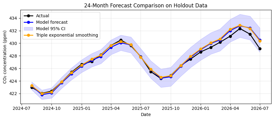
Figure 10: SARIMA and Triple Exponential Smoothing forecasts compared with actual observations.
From Figure 10 we see that Triple Exponential Smoothing also performs remarkably well on the unseen observations. Its forecasts closely follow the actual CO2 concentrations throughout the validation period and reproduce both the upward trend and annual seasonal cycle. The SARIMA and Triple Exponential Smoothing forecasts are also extremely close to one another. In many months, the difference between the two predictions is only a few hundredths or tenths of a ppm.
This agreement is particularly interesting because the two models approach the forecasting problem from different mathematical perspectives. SARIMA captures autocorrelation and seasonal dependence through AR and MA structures, whereas Holt-Winters captures the evolving level, trend, and seasonality directly.
The similarity of their predictions therefore suggests that the dominant structure in the CO2 series is strong, persistent, and consistently identifiable across different modelling approaches, making atmospheric CO2 concentrations highly predictable.
Forecast accuracy was also assessed more formally using the Mean Absolute Error (MAE) and Root Mean Squared Error (RMSE). The results over the validation period showed that both models performed remarkably well, with neither method demonstrating a meaningful superiority over the other. This indicates that both models were highly effective at reproducing the underlying trend and seasonal cycle throughout the validation period. A more detailed account of this analysis is provided in the accompanying notebook.
7. Generating a 5-Year Forecast
Following the successful out-of-sample validation, the selected SARIMA model was re-estimated using the complete available CO2 dataset. This allows the final forecasting model to incorporate all observations available up to July 2026 before generating predictions for the following five years.
The re-estimated model produces a log-likelihood of -198.738, with an AIC of 419.476,
a BIC of 469.908, and an HQIC of 438.941. The parameter estimates remain highly
consistent with those obtained from the training sample. Both non-seasonal MA terms remain statistically significant, while the seasonal AR coefficients
retain the same overall pattern, with significant dependence at annual multiples.
The similarity between the parameter estimates from the training-sample model and the full-sample model provides additional evidence that the selected
SARIMA specification is stable when additional observations are incorporated.
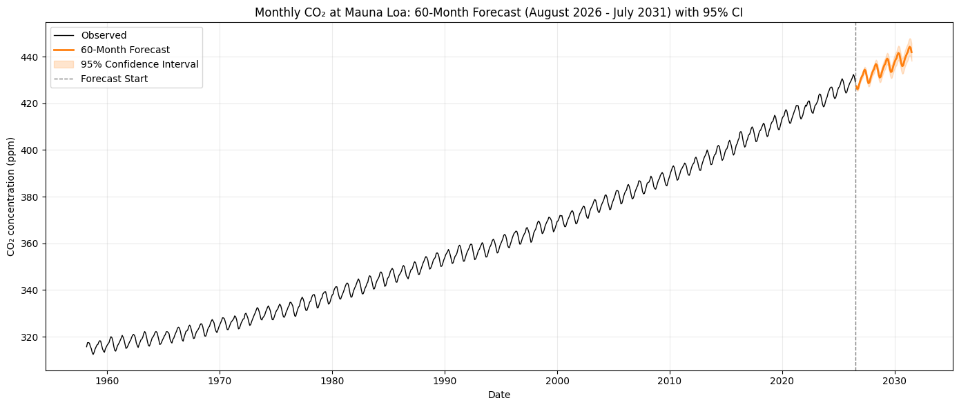
Figure 11: Monthly Atmospheric CO2 Concentrations at Mauna Loa: 5 Years Forecast (August 2026 - July 2031)
Using this refitted model, forecasts were generated for the next 60 months, covering the period from August 2026 through July 2031. The forecasts showcase a continued long-term upward trajectory, consistent with the trend observed throughout the historical series, while retaining the pronounced annual seasonal cycle. The highest forecasted concentration is approximately 444.22 ppm in May 2031.
8. Conclusion
Overall, the Mauna Loa atmospheric CO2 series provides an excellent example of how a complete time-series analysis and forecasting workflow can be applied to a real-world environmental dataset. This analysis demonstrates the complete journey from a raw environmental time series to a validated forecasting model, with each stage carried out systematically and step by step:
- Explore the raw series to identify trend and seasonality.
- Examine ACF and PACF to understand temporal dependence.
- Apply ADF and KPSS tests to assess stationarity formally.
- Difference the series when required to remove non-stationary behaviour.
- Use ACF and PACF to generate candidate time-series models.
- Compare models using AIC, BIC, parameter significance, and residual diagnostics.
- Validate forecasts chronologically using observations excluded from model estimation.
- Compare against alternative forecasting methods such as Triple Exponential Smoothing.
We conclude this analysis with comments on the remarkably good forecasting performance observed on the unseen dataset. The models performed exceptionally well during validation, which is not always the case in real-world forecasting problems. A plausible explanation for this strong generalisation lies in the nature and construction of the CO2 dataset itself. The published Mauna Loa CO2 series is a processed observational product rather than a direct stream of unprocessed sensor measurements.
The dataset undergo substantial quality control, screening, and processing before publication. As a result, the final monthly series is considerably cleaner and more structured than raw sensor output would typically be. This preprocessing and smoothing contribute to a time series with a strong and persistent underlying structure, characterised primarily by a clear long-term upward trend and a pronounced annual seasonal cycle. These features make the series highly predictable and allow statistical forecasting models to generalise effectively to unseen observations.