Introduction
In the previous analysis, a comprehensive statistical time-series analysis workflow was used to model and forecast atmospheric CO2 concentrations, with the selected models generalizing well to unseen observations and performing strongly on the holdout data. In this analysis, we turn to another important greenhouse gas, methane (CH4), but instead of statistical time-series methods, we explore how a range of machine-learning methods can be applied to the forecasting problem.
The dataset was obtained from the National Oceanic and Atmospheric Administration (NOAA) and is based on observations from marine surface monitoring sites. It contains globally averaged monthly mean atmospheric CH4 concentrations expressed in parts per billion (ppb). The available dataset contains 514 monthly observations spanning July 1983 to April 2026.
The analysis follows a standard machine-learning workflow consisting of exploratory data analysis, feature engineering, model development, hyperparameter tuning, model evaluation, and forecasting. However, a key characteristic of this analysis is that the forecasting problem is formulated as a univariate machine-learning problem. No external explanatory variables are supplied to the models. Instead, the models must learn from the historical behaviour of the CH4 series itself.
This makes appropriate feature engineering particularly important, including the construction of lagged predictors from the historical series and the incorporation of other time-derived features. These engineered variables will provide a conventional supervised-learning model with information about temporal dependencies and recurring patterns within the CH4 series. The approach adopted in this study is described later in the feature-engineering section.
Given the univariate nature and pronounced temporal patterns of the series, we focus on relatively structured supervised machine-learning approaches, including Ordinary Least Squares (OLS), Ridge Regression, Lasso Regression, Elastic Net Regression, alongside a Support Vector Regression (SVR) model with an Radial Basis Function (RBF) kernel. More complex machine-learning approaches, such as tree-based ensembles and deep neural networks, often do not produce better forecasting performance for relatively simple, strongly structured univariate series and are therefore not considered here. The selected models and their characteristics are discussed in the following sections.
- This article focuses on the practical forecasting workflow, modelling decisions, and interpretation of results. It is not intended to provide a complete theoretical treatment of every machine-learning algorithm or mathematical derivation.
- For those interested in the technical implementation, a fully documented Jupyter Notebook is provided in this GitHub repository. It contains all code, outputs, figures, and detailed Markdown explanations supporting the analysis. The repository also includes the Notebook from the previous CO2 time-series study.
1. Data Analysis
We begin with an exploratory analysis of the CH4 series. The purpose of this stage is to understand the main temporal characteristics of the data before constructing machine-learning features. In particular, we examine the long-term movement of the series, its seasonal behaviour, month-to-month changes, and autocorrelation structure.
1.1 Raw CH4 Series Inspection
The raw global monthly mean CH4 concentration series is first examined by plotting the
average variable provided in the datasets. As shown in Figure 1, atmospheric methane exhibits a clear
long-term upward trend. Concentrations rise from approximately
1626 ppb in 1983 to 1937 in April 2026,
representing a substantial increase over the four-decade observation period. Alongside this long-term trend, the series exhibits
a noticeable within-year seasonal pattern, with concentrations regularly fluctuating throughout the year.
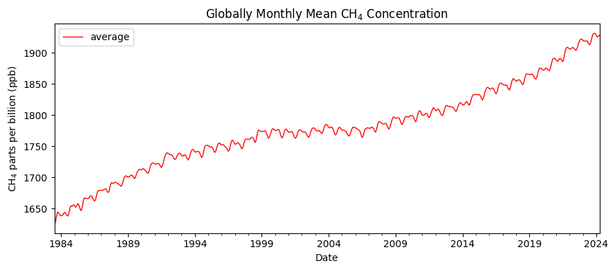
Figure 1: Globally averaged monthly atmospheric CH4 concentrations over the observation period.
One particularly interesting period occurs between approximately 1999 and 2006, when the overall increase in atmospheric methane appears to slow substantially or temporarily stabilize. This period corresponds to a well-documented global methane growth plateau observed around the early 2000s. After this period, the upward trajectory resumes, with the increase becoming more pronounced in recent years.
Overall, the raw series contains three features that are especially important for subsequent modelling: a strong long-term trend, recurring annual variation, and a period of slower growth during the early 2000s. These characteristics provide the starting point for the feature-engineering strategy developed later in the article.
1.2 Regular Differencing
To examine the month-to-month dynamics separately from the long-term level, regular first differencing is applied with a lag of one month. Rather than describing the concentration itself, the differenced series describes how much the concentration changed compared with the previous month:
\[ \Delta CH_{4,t} = CH_{4,t}-CH_{4,t-1}. \]In simple terms, a positive value means that atmospheric CH4 increased relative to the previous month, while a negative value means that it decreased. This transformation is useful during exploratory analysis because it reduces the dominant long-term trend and makes shorter-term and seasonal movements easier to inspect.
1.3 ACF and PACF of the Regularly Differenced Series
The autocorrelation function (ACF) and partial autocorrelation function (PACF) are examined after regular first differencing. The ACF measures the relationship between the current value and previous values at different lags, while the PACF measures the relationship at a particular lag after accounting for shorter lagged relationships.
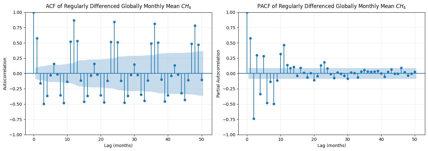
Figure 2: ACF and PACF of the regularly differenced CH4 series.
ACF Observations
As shown in Figure 2, the ACF reveals a pronounced seasonal structure at multiples of 12 months. Lag 1 shows statistically significant positive autocorrelation, while strong positive autocorrelation also appear at lags 12, 24, 36, and 48. This indicates that annual temporal structure remains clearly visible even after the long-term trend has been reduced through first differencing.
Additional structure is visible at several shorter intra-year lags. In particular, some lags separated by approximately six months (3, 9, 15, 21, 27, 33, ...) exhibit negative autocorrelation. This alternating pattern suggests that the month-to-month changes in atmospheric methane contains a repeating intra-year structure rather than simply a straightforward annual cycle. The alternating positive and negative correlations suggest that observations at certain positions within the seasonal cycle tend to move in opposite directions.
PACF Observations
The PACF provides a complementary view of the dependence structure. Several of the first 12 lags exhibit statistically meaningful partial autocorrelation, indicating that the short-term dynamics cannot be described adequately using only the immediately preceding observation.
Taken together, the ACF and PACF provide an empirical basis for the feature-engineering stage. They suggest that recent observations and seasonal relationships are likely to contain useful predictive information.
Implications for Feature Engineering
The correlation analysis does not imply that every statistically significant lag should automatically become a machine-learning feature. Many lagged variables are strongly related to one another, and including too many can introduce redundancy and unnecessary complexity. Instead, the ACF and PACF results are used as a data-informed starting point.
The candidate feature set therefore includes three broad forms of historical information:
- Short-term lags: recent observations such as one- and two-month lags that capture immediate persistence and short-term movement.
- Annual seasonal lags: particularly the 12-month lag, which allows the model to compare the current seasonal position with the corresponding period in the previous year.
- Rolling and aggregated features: rolling means, standard deviations, and short-term trend measures that summarize recent levels and variability.
1.4 Monthly Distribution of Differenced CH4
To investigate the seasonal pattern more directly, the regularly differenced CH4 series is grouped by calendar month. The resulting boxplot describes the distribution of month-to-month changes in January, February, March, and so on.
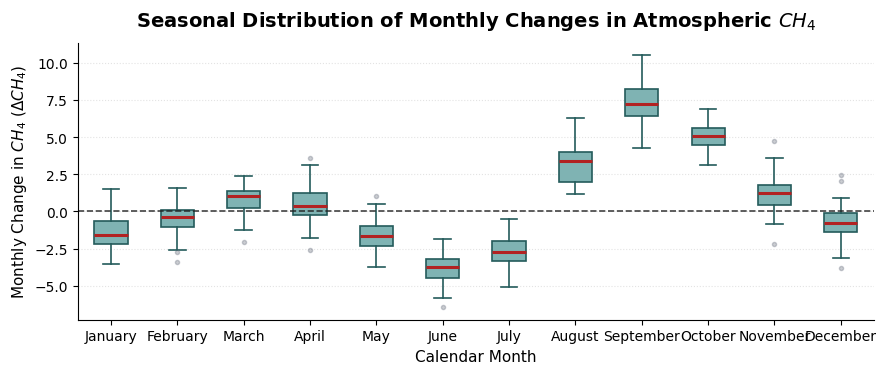
Figure 3: Distribution of month-to-month CH4 changes by calendar month.
As shown in Figure 3, the monthly changes are not distributed uniformly across the calendar year. From approximately January through April, the distributions remain relatively close to zero. A stronger negative movement then appears in May and June, with June showing the most pronounced negative median change. The pattern subsequently reverses during late summer and early autumn. August and September exhibit strong positive median changes, with September showing the largest positive median increase. Positive movement remains visible in October before weakening substantially later in the year.
The strongest departures from zero therefore occur between approximately May and October. This provides additional evidence that the methane series contains a substantial within-year seasonal component. The result also supports the inclusion of calendar and seasonal features in the forecasting models.
A positive median does not mean that atmospheric CH4 concentration is necessarily highest during that month. Rather, it indicates that CH4 concentrations tend to increase relative to the preceding month. Likewise, a negative median indicates a tendency for concentrations to decrease relative to the previous month. This reflects the fact that seasonal changes in atmospheric CH4 are influenced by multiple processes whose strength and timing can vary over time. These include natural sources, such as wetlands, which respond to temperature and hydrological conditions, as well as anthropogenic sources, including agriculture, livestock, waste management, and energy production.
2. Feature Engineering and Feature Selection
The objective of feature engineering is to transform the univariate global monthly CH4 series into a supervised-learning problem while preserving the chronological forecasting structure and avoiding data leakage. The exploratory analysis identified three main sources of predictive information: recent temporal dependence, annual seasonality, and short-term changes in the series. These findings motivate the construction of calendar variables, lagged observations, historical differences, seasonal differences, rolling statistics, and local trend measures.
For each month \(t\), the target variable (represented by average in our dataset) is;
\(y_t = CH_4(t),\) while the feature vector contains information that would have been available before the
target month was observed. A relatively broad candidate set is initially generated. This allows potentially useful temporal information to
be considered, however, the final feature selection is based on out-of-sample performance within the training data.
2.1 Forecasting Information Set and Leakage Prevention
In a forecasting problem, the value of the target variable at time \(t\) is unknown when the prediction is made. This means, every predictor must be constructed using observations from time \(t-1\) or earlier. The general forecasting relationship can therefore be written as:
where \(f(\cdot)\) represents the feature-engineering transformations. This restriction prevents data leakage. For example, the current difference; \(y_t-y_{t-1},\) cannot be used to predict \(y_t,\) because it already contains the value being predicted. Instead, a valid historical difference is constructed entirely from previously observed values: \(\Delta_{1,t}=y_{t-1}-y_{t-2}.\) The same principle applies to rolling statistics:
The auxiliary variables from the original dataset average_unc, trend, and
trend_unc are not included in the machine-learning feature matrix.
The modelling problem therefore remains strictly univariate, with all predictive information
derived from the historical CH4 concentration series and known calendar information.
2.2 Calendar and Cyclical Features
Calendar information is known at the time of forecasting and can therefore be used without leakage.
The original features set included year, month, and decimal, with
calendar information represented numericaly. However, treating month as an ordinary numerical variable may
incorrectly imply that December (12) and January (1) are far apart.
To avoid this, month is represented both directly and using cyclical transformations:
These features allow the models to represent the continuous transition from one calendar year into the next. Moreover, the inclusion of these features is directly motivated by the monthly boxplot analysis. The differenced CH4 series showed substantial differences between calendar months, with strongly negative median changes during June and July and strongly positive changes during August, September, and October.
2.3 Lagged Concentration Features
Lagged observations form the core of the univariate forecasting framework. They provide direct information about previous methane concentrations and allow the model to learn how the future value relates to the recent history of the series.
The exploratory ACF and PACF analysis provided empirical guidance for constructing candidate
lags. The initial set included short-term lags such as
lag_1, lag_2, lag_3, and lag_9 together with the annual
seasonal lags lag_12, lag_24, lag_36 and lag_48:
The short lags provide information about recent concentration levels, while lags around 12 months and its multiples captures persistence relative to the corresponding seasonal position in the previous year.
2.4 Historical Change Features
The differenced-series analysis showed that month-to-month methane changes contain useful temporal structure. Historical change features therefore provide the model with information about recent momentum. To avoid leakage, these changes are calculated only from previously observed values. For example:
These features allow the model to use information about not only the current historical
level of methane but also the direction and magnitude of recent changes.
Several short-term and longer-term historical differences are initially considered, including diff_lag_12.
Their final inclusion is determined by the subsequent feature-selection process.
2.5 Historical Seasonal-Difference Features
Seasonal-difference features describe how recent methane concentrations compare with the corresponding period one year earlier. For example:
This compares the most recently observed month with the same seasonal position one year earlier (year-over-year changes). Similar features are constructed for previous lags. These variables were motivated by the annual autocorrelation structure shown in Figure 3. They provide a direct measure of whether recent methane levels are above or below the corresponding seasonal levels observed during the previous year.
2.6 Rolling Statistics
Rolling statistics summarize recent observations and provide information that may not be
represented clearly by a single lag. Candidate windows represented short and annual-scale behaviour,
including 3-month, and 12-month windows. For a window of \(k\) months,
For example a 3-month rolling mean is defined as:
Rolling standard deviations are also calculated using the same historical observations. A rolling mean summarizes the recent methane level, while a rolling standard deviation provides information about the recent variability of the series.
2.7 Short-Term Trend Features
To complement the raw lagged differences, additional trend features are constructed from differences between historical rolling means. For example:
These variables provide a smoothed explicit measure of short-term direction by comparing the most recent historical average level with a slightly longer historical average.
2.8 From Candidate Features to the Final Feature Set
The feature-engineering process deliberately begins with a relatively broad set of candidate predictors. However, several engineered features contain overlapping information. Adjacent lags are often strongly correlated, rolling means are mathematical combinations of lagged observations, and seasonal differences are themselves constructed from historical lags. Retaining every candidate feature would therefore increase dimensionality without necessarily adding useful predictive information.
Because of this, feature selection was treated as an empirical modelling decision. Candidate features were evaluated through a series of chronological model-development experiments, with individual variables or feature groups removed when their inclusion did not improve validation performance. As a result, the final feature matrix was reduced from the broader candidate set to 18 predictors. The retained variables represent complementary information from several parts of the historical series:
-
Calendar seasonality:
month,month_sin, andmonth_cos. -
Recent concentration levels:
lag_1,lag_2, andlag_12. -
Recent historical changes:
diff_lag_1,diff_lag_2,diff_lag_3, anddiff_lag_12. -
Year-over-year behaviour:
seasonal_diff_lag_1andseasonal_diff_lag_2. -
Recent level and variability:
rolling_mean_3,rolling_mean_12, androlling_std_12. -
Short-term trend:
trend_1_2,trend_2_3, andtrend_3_6.
The resulting feature set is consequently smaller but more targeted. Rather than attempting to represent every temporal relationship detected during exploratory analysis, it focuses on features that demonstrated useful predictive information in the supervised-learning framework.
3. Linear Regression Models
The first group of forecasting models consists of Ordinary Least Squares (OLS), Ridge, Lasso, and Elastic Net regression. All four models predict the target from the engineered feature matrix, but they differ in how the regression coefficients are estimated and constrained.
Let \(p\) denote the number of predictors and \(n\) the number of training observations. The supervised-learning problem can be written in matrix form as: \(\mathbf{y}=\mathbf{X}\boldsymbol{\beta}+\boldsymbol{\varepsilon},\) where;
\(\mathbf{y}\) contains the observed methane concentrations, \(\mathbf{X}\) contains the engineered predictors, \(\boldsymbol{\beta}=(\beta_0,\beta_1,\ldots,\beta_p)^T\) contains the intercept and predictor (model) coefficients, and \(\boldsymbol{\varepsilon}\) represents the remaining prediction error.
The principal difference between the models is how they estimate \(\boldsymbol{\beta}\). OLS minimizes prediction error alone, whereas Ridge, Lasso, and Elastic Net add penalties that constrain coefficient magnitude. These regularization methods are particularly relevant because many predictors are derived from the same underlying CH4 series and may therefore be correlated.
3.1 Ordinary Least Squares (OLS)
OLS estimates the coefficients that minimize the sum of squared prediction errors. For an individual observation:
In matrix form, \(\hat{\mathbf y}=\mathbf X\boldsymbol{\beta}\). The coefficients are obtained by solving:
\[ \hat{\boldsymbol{\beta}}_{\mathrm{OLS}} = \arg\min_{\boldsymbol{\beta}} \left\| \mathbf{y} - \mathbf{X}\boldsymbol{\beta} \right\|_2^2, \]where \(\|\cdot\|_2^2\) denotes the sum of squared residuals. When \(\mathbf X^T\mathbf X\) is invertible, the solution has the familiar closed form;
\[ \hat{\boldsymbol{\beta}}_{\mathrm{OLS}} = (\mathbf X^T\mathbf X)^{-1}\mathbf X^T\mathbf y. \]OLS provides an important baseline because it evaluates the predictive value of the engineered features without coefficient regularization. However, predictors derived from a time series can be highly correlated. For example, nearby lags and rolling statistics contain overlapping information. This multicollinearity can make individual OLS coefficients unstable, even when the model's predictions remain useful. Regularized regression is therefore considered as an alternative.
3.2 Ridge Regression
Ridge regression extends OLS by penalizing large coefficients. It uses an an \(L_2\) penalty, which is based on the squared magnitude coefficients:
\[ \left\| \boldsymbol{\beta} \right\|_2^2 = \sum_{j=1}^{p}\beta_j^2. \]The Ridge objective function can be written as:
Equivalently, it has a closed form;
\[ \hat{\boldsymbol{\beta}}_{\mathrm{Ridge}} = (\mathbf X^T\mathbf X + \lambda I)^{-1}\mathbf X^T\mathbf y. \]The parameter \(\lambda\geq0\) controls the strength of regularization. When \(\lambda=0\), the objective reduces to OLS. As \(\lambda\) increases, larger coefficients are penalized more strongly and are therefore shrunk toward zero. The purpose of this shrinkage is not necessarily to eliminate predictors, but to reduce the influence of unstable or highly correlated coefficients. This makes Ridge particularly relevant to the present feature set, where several lagged and aggregated variables may contain overlapping information. The intercept is not penalized. Because the penalty depends on the scale of the predictors, the features are usually standardized within the modelling pipeline before fitting Ridge.
3.3 Lasso Regression
Lasso (Least Absolute Shrinkage and Selection Operator) uses an \(L_1\) penalty, defined as the sum of the absolute values of the coefficients:
\[ \left\| \boldsymbol{\beta} \right\|_1 = \sum_{j=1}^{p} |\beta_j|. \]Its objective function is:
Unlike Ridge, the \(L_1\) penalty can produce coefficients that are exactly zero. This means, Lasso performs both coefficient shrinkage and implicit feature selection. This property is useful for the present problem because the engineered feature set contains predictors that may provide overlapping information. By driving the coefficients of less informative predictors to zero, Lasso can therefore produce a more compact and interpretable model.
However, when several predictors are strongly correlated, Lasso may favour one predictor over others in the correlated group rather than retaining all of them. This can result in the exclusion of potentially valuable information and may make the selected features less stable.
- Unlike OLS and Ridge, Lasso generally does not have a closed-form matrix solution. The reason is that the \(L_1\) penalty \(|\beta_j|\) is not differentiable at \(0\).
- Instead, Lasso is typically solved using numerical optimization methods such as coordinate descent. These methods are usually used to find the bounded optimum and they can produce coefficients that are exactly zero, allowing Lasso to perform variable selection.
3.4 Elastic Net Regression
Elastic Net combines the \(L_1\) penalty used by Lasso with the \(L_2\) penalty used by Ridge. Its objective can be expressed conceptually as:
where \(\lambda\) controls the overall regularization strength and \(\alpha\in[0,1]\) determines the relative contribution of the two penalties. Therefore:
- \(\alpha=1\) gives the Lasso penalty;
- \(\alpha=0\) gives the Ridge penalty;
- \(0 < \alpha < 1\) balances the two forms of regularization.
Elastic Net is particularly relevant when the feature matrix contains both correlated predictors and potential redundancy. The \(L_1\) regularization component remove weak predictors, while the \(L_2\) component provides coefficient shrinkage and help distribute information across correlated predictors rather than forcing an arbitrary single choice. Both \(\lambda\) and \(\alpha\) are therefore tuned during model development.
- The squared-error loss may be written using different constant factors, for example \[ \|\mathbf y-\mathbf X\boldsymbol{\beta}\|_2^2, \quad \frac{1}{2}\|\mathbf y-\mathbf X\boldsymbol{\beta}\|_2^2, \quad \frac{1}{n}\|\mathbf y-\mathbf X\boldsymbol{\beta}\|_2^2, \quad \frac{1}{2n}\|\mathbf y-\mathbf X\boldsymbol{\beta}\|_2^2. \] These are scaling conventions and do not change the underlying type of regularization.
- The numerical value of \(\lambda\) depends on the scaling convention used. Therefore, when the loss is rescaled, the regularization parameter must be interpreted or rescaled consistently.
- One of the most commonly introduced factor is \(1/2\). It is commonly used because it simplifies differentiation of the squared-error term by removing the otherwise resulting factor of \(2\): \[ \nabla_{\boldsymbol{\beta}} \left( \frac{1}{2}\|\mathbf y-\mathbf X\boldsymbol{\beta}\|_2^2 = \frac{1}{2}(y-X\beta)^T(y-X\beta) \right) = -\mathbf X^T(\mathbf y-\mathbf X\boldsymbol{\beta}), \]
- When the \(1/2\) convention is used, the three regularized objectives become: \[ \text{Ridge:}\qquad \min_{\boldsymbol{\beta}} \frac{1}{2}\|\mathbf y-\mathbf X\boldsymbol{\beta}\|_2^2 +\frac{\lambda}{2}\|\boldsymbol{\beta}\|_2^2, \] \[ \text{Lasso:}\qquad \min_{\boldsymbol{\beta}} \frac{1}{2}\|\mathbf y-\mathbf X\boldsymbol{\beta}\|_2^2 +\lambda\|\boldsymbol{\beta}\|_1, \] and \[ \text{Elastic Net:}\qquad \min_{\boldsymbol{\beta}} \frac{1}{2}\|\mathbf y-\mathbf X\boldsymbol{\beta}\|_2^2 +\lambda \left( \alpha\|\boldsymbol{\beta}\|_1 +\frac{1-\alpha}{2}\|\boldsymbol{\beta}\|_2^2 \right). \] Thus, the \(1/2\) is simply attached to the squared-error term; it does not change the type of regularization being used.
- Throughout, we used the unscaled squared-error convention: \(\|\mathbf y-\mathbf X\boldsymbol{\beta}\|_2^2.\)
4. Support Vector Regression with an RBF Kernel
The linear models assume that the relationship between the engineered predictors and future CH4 concentration can be represented as a weighted linear combination of the features. However, temporal and seasonal relationships may contain nonlinear interactions.
Support Vector Regression (SVR) provides a nonlinear alternative. Rather than relying only on a linear relationship in the original feature space, SVR can use a kernel function to model more flexible relationships between observations. In this analysis, a Radial Basis Function (RBF)-kernel SVR is used to determine whether additional nonlinear flexibility improves forecasting performance.
4.1 Support Vector Regression
Support Vector Regression (SVR) is an extension of Support Vector Machines that can be used to solve regression problems. For a linear SVR, the prediction function can be written as: \(f(\mathbf{x})=\mathbf{x}^{T}\boldsymbol{\beta}+b.\) SVR seeks a function that is sufficiently flat while keeping prediction errors within an \(\epsilon\)-wide tolerance region whenever possible. For an observation \((\mathbf{x}_i,y_i)\), an error is considered acceptable when:
\[ |y_i-f(\mathbf{x}_i)| \leq \epsilon. \]Thus, errors inside the interval \([f(\mathbf{x}_i)-\epsilon,\;f(\mathbf{x}_i)+\epsilon]\) are not penalized. This is known as the \(\epsilon\)-insensitive loss. When an observation falls outside this interval, only the amount by which the error exceeds \(\epsilon\) is penalized:
\[ L_{\epsilon}(y_i,f(\mathbf{x}_i)) = \max \left( 0, |y_i-f(\mathbf{x}_i)|-\epsilon \right). \]The parameter \(\epsilon\) therefore controls the width of the tolerance region. A larger \(\epsilon\) allows larger deviations between predictions and observations before a penalty is applied, whereas a smaller \(\epsilon\) requires predictions to remain closer to the observed values.
4.2 SVR Regularization
SVR balances two competing objectives: producing a relatively simple prediction function while limiting prediction errors outside the \(\epsilon\)-insensitive region. For the linear case, the optimization problem can be written as:
\[ \min_{\boldsymbol{\beta},b,\xi_i,\xi_i^*} \|\boldsymbol{\beta}\|_2^2 + C\sum_{i=1}^{n}(\xi_i+\xi_i^*) \] subject to \[ y_i-\left(\mathbf{x}_i^T\boldsymbol{\beta}+b\right) \leq \epsilon+\xi_i, \] \[ \left(\mathbf{x}_i^T\boldsymbol{\beta}+b\right)-y_i \leq \epsilon+\xi_i^*, \] \[ \xi_i,\xi_i^*\geq0. \]The variables \(\xi_i\) and \(\xi_i^*\) represent deviations beyond the \(\epsilon\)-insensitive region. The parameter \(C\) determines how strongly these deviations are penalized. A large \(C\) places greater emphasis on fitting the training observations and therefore allows less tolerance for errors outside the \(\epsilon\) region. A small \(C\) imposes stronger regularization, allowing more training error in exchange for a smoother, less complex fitted function. Thus, \(C\) controls the trade-off between fitting the training data and controlling model complexity.
4.3 The Radial Basis Function (RBF) Kernel
The nonlinear capability of the model comes from the kernel function. Rather than explicitly creating a large number of nonlinear transformations and interaction terms, SVR uses a kernel to measure the similarity between observations. One of the kernel the model uses is the Radial Basis Function (RBF) kernel. The RBF kernel is defined as:
\[ K(\mathbf{x}_i,\mathbf{x}_j) = \exp \left( -\gamma \left\| \mathbf{x}_i-\mathbf{x}_j \right\|_2^2 \right). \] where \[ \|\mathbf{x}_i-\mathbf{x}_j\|_2^2 = \sum_{k=1}^{p} (x_{ik}-x_{jk})^2 \]This is the squared Euclidean distance between two observations in the feature space. The kernel therefore assigns a value between 0 and 1 according to how similar the two observations are:
- Observations that are close together have a kernel value close to 1;
- Observations that are far apart have a kernel value approaching 0.
The parameter \(\gamma\) controls how quickly this similarity decreases with distance. A small \(\gamma\) produces a broader region of influence, resulting in a smoother and less flexible relationship. A large \(\gamma\) produces a narrower region of influence, allowing the model to respond to more localized patterns. \(\gamma\) therefore controls the local flexibility of the nonlinear relationship.
4.4 RBF-SVR Prediction Function
With the RBF kernel, the fitted prediction function can be represented as:
\[ f(\mathbf{x}) = \sum_{i=1}^{n} (\alpha_i-\alpha_i^*) K(\mathbf{x}_i,\mathbf{x}) +b, \]where the coefficients \((\alpha_i-\alpha_i^*)\) determine the contribution of the training observations and \(b\) is the intercept. Substituting the RBF kernel gives:
This formulation illustrates how the nonlinear model makes predictions. Conceptually, a new observation receives influence from training observations according to their similarity in the engineered feature space. For the present forecasting problem, this means that a historical pattern involving; recent CH4 levels, seasonal position, recent changes, and rolling statistics can have a similar influence on a new month when those features are jointly similar. The model can therefore capture nonlinear combinations of the engineered predictors without explicitly constructing interaction terms.
4.5 SVR Hyperparameters
The RBF-SVR has three main hyperparameters that determine its behaviour:| Parameter | Role | Effect of Increasing the Value |
|---|---|---|
| \(C\) | Controls the penalty for errors outside the \(\epsilon\)-tube | Places greater emphasis on fitting the training data |
| \(\epsilon\) | Defines the width of the error tolerance region | Allows larger errors before they are penalized |
| \(\gamma\) | Controls how rapidly similarity decreases with distance | Produces more localized and flexible nonlinear relationships |
As summarized in Table 1, these parameters interact with one another. For example, a large \(C\) combined with a large \(\gamma\) can produce a highly flexible model that follows localized patterns closely, whereas smaller values generally produce a smoother relationship. Their values must therefore be determined empirically through chronological validation rather than selected independently.
- In some formulations \( \mathbf{x}^T\boldsymbol{\beta} \) is sometimes written as \( \boldsymbol{\beta}^T\mathbf{x} \). These are equivalent because their result is a scalar: \[ \mathbf{x}^T\boldsymbol{\beta} = \boldsymbol{\beta}^T\mathbf{x}. \] This follows from the commutative property of matrix transpose. If you want a deeper explanation, see this linear algebra blog post .
- Additionally, you may see the regularization term written as either \[ \frac{1}{2}\|\boldsymbol{\beta}\|^2, \quad\text{instead of;}\quad \|\boldsymbol{\beta}\|^2. \] The factor \( \frac{1}{2} \) is mainly a mathematical convenience because it makes differentiation simpler. It does not fundamentally change the optimization problem when the other terms, such as \(C\), are scaled consistently. Thus, different sources may use different conventions.
5. Model Evaluation Metrics
Model performance is evaluated using four complementary metrics: MAE, RMSE, \(R^2\), and MAPE. Each metric provides a different perspective on predictive performance.
5.1 Mean Absolute Error (MAE)
\[ MAE = \frac{1}{n} \sum_{t=1}^{n} |y_t-\hat{y}_t|. \]MAE measures the average absolute forecasting error. It is expressed in the same units as the target, in this case; the target is atmospheric methane concentration expressed in parts per billion (ppb), MAE is therefore expressed directly in ppb. Lower MAE indicates better predictive accuracy.
5.2 Root Mean Squared Error (RMSE)
\[ RMSE = \sqrt{ \frac{1}{n} \sum_{t=1}^{n} (y_t-\hat{y}_t)^2 }. \]Like MAE, RMSE is also expressed in ppb, but it gives greater weight to larger forecasting errors because the errors are squared before averaging. Comparing RMSE with MAE can therefore provide insight into whether a model occasionally produces relatively large deviations.
5.3 Coefficient of Determination (\(R^2\))
\[ R^2 = 1- \frac{ \sum_{t=1}^{n}(y_t-\hat{y}_t)^2 }{ \sum_{t=1}^{n}(y_t-\overline{y})^2 }. \]\(R^2\) measures the proportion of variation in the observed target explained by the predictions relative to a constant-mean prediction. Values closer to \(1\) indicate that the predictions explain more of the observed variation relative to the mean baseline. An \(R^2\) of \(0\) corresponds to performance equivalent to predicting the sample mean, while negative values indicate performance worse than that baseline.
5.4 Mean Absolute Percentage Error (MAPE)
\[ MAPE = \frac{100}{n} \sum_{t=1}^{n} \left| \frac{y_t-\hat{y}_t}{y_t} \right|. \]MAPE expresses the absolute error relative to the observed value. It provides an intuitive percentage-based measure of error. MAPE can be problematic when observed values are zero or close to zero because the denominator becomes unstable. This is not a practical issue for atmospheric CH4 concentrations, which remain far above zero throughout the dataset.
5.5 Metric Interpretation
MAE and RMSE are the primary forecasting metrics because they express errors directly in ppb. MAE gives equal importance to all errors, whereas RMSE places greater emphasis on larger errors. \(R^2\) provides a relative measure of explained variation, while MAPE expresses typical forecasting error on a percentage scale.
| Metric | What It Measures | Preferred Direction |
|---|---|---|
| MAE | Average absolute forecasting error in ppb | Lower |
| RMSE | Error magnitude with greater emphasis on large deviations | Lower |
| R2 | Explained variation relative to a mean baseline | Higher |
| MAPE | Average relative forecasting error expressed as a percentage | Lower |
As summarized in Table 2, no single metric captures every aspect of forecasting performance. The models are therefore evaluated using multiple measures rather than relying on one statistic alone.
6. Cross-Validation, Hyperparameter Tuning and Feature Scaling
6.1 Time-Series Cross-Validation
Since the objective of the analysis is to evaluate forecasting performance on a chronological time series, the sequential structure of the data must be preserved throughout model development. Random train-test splits are inappropriate for this setting because they may allow observations from later periods to enter the training data while earlier periods are being evaluated. This can lead to data leakage and overly optimistic estimates of out-of-sample forecasting performance.
Instead, all five models—OLS, Ridge, Lasso, Elastic Net, and RBF-SVR—are evaluated using expanding-window time-series cross-validation. Under this approach, the training sample grows sequentially through time, while each validation period occurs strictly after the corresponding training period. This procedure more closely reflects the actual forecasting problem, where future observations cannot be used during model training or model selection. A simplified representation of the expanding-window procedure is:
6.2 Feature Scaling
In all models feature standardization is performed
within the Pipeline, using StandardScaler() from sklearn.preprocessing. Feature scaling is particularly important for the RBF-SVR because the kernel depends directly on the distances
between observations:
If one predictor has a substantially larger numerical scale than another, it can dominate the distance calculation
and consequently dominate the kernel similarity. Scaling is also important for Ridge, Lasso and Elastic Net,
because their fitted parameters are sensitive to the scale of the predictors. However,
for ordinary linear regression, scaling isn't strictly necessary, although it can still be useful for numerical stability
and making coefficients more comparable. For each feature/column, StandardScaler() transforms the values using:
where, \(x_{ij}\) is the original value, \(\mu_j\) is the mean of that feature in the training data, \(\sigma_j\) is the standard deviation of that feature in the training data, and \(z_{ij}\) is the scaled value. After scaling, each feature is approximately \(\mu=0\) and \(\sigma=1\). The scaler is placed inside the modelling pipeline so that it is fitted separately within each chronological training fold. This ensures that validation observations do not influence the scaling parameters.
6.3 Hyperparameter Tuning Across Models
The extent of hyperparameter tuning differs across the five models. The OLS model is an unregularized linear benchmark and therefore has no regularization or kernel hyperparameters to optimise. Ridge, Lasso, and Elastic Net introduce regularization parameters, while RBF-SVR additionally contains kernel-specific parameters. Hyperparameter selection is therefore performed separately for each model using the same chronological cross-validation framework.
For the OLS model, no hyperparameters are tuned. OLS therefore provides an unregularized linear benchmark against which the effects of regularization and
nonlinear modelling can be assessed. For Ridge regression, the regularization strength \(\lambda\) is tuned, whereby a predefined grid of
candidate \(\lambda\) values is evaluated across the chronological validation folds. For Lasso regression, the regularization strength \(\lambda\) is likewise
selected through chronological cross-validation. As for Elastic Net, two hyperparameters are tuned: the overall regularization
strength \(\lambda\) and the l1-ratio, denoted by \(\alpha\).
In the RBF-SVR model, values of hyperparameters \(C\), \(\epsilon\), and \(\gamma\) determine the balance between fitting accuracy, tolerance to error, and nonlinear flexibility. They are therefore selected using the same five-fold expanding-window cross-validation framework used for the linear models. A predefined grid of candidate values is evaluated for these three hyperparameters, and the combination that provides the best cross-validated forecasting performance is selected.
For each candidate hyperparameter configuration, the model is fitted using the training observations of each chronological fold and evaluated on the subsequent validation period. Forecasting performance is measured using MAE, RMSE, \(R^2\), and MAPE.
7. Model Results and Discussion
The preceding sections established the forecasting framework, feature-engineering strategy, candidate models, validation procedure, and evaluation metrics. The next stage compares the fitted models using chronological validation and the final holdout data. The complete implementation, tuning procedure, model outputs, additional figures and detailed Markdown explanations can be examined in the accompanying Jupyter Notebook.
7.1 Chronological Cross-Validation Results
The cross-validation results are summarized in Table 3. All five models achieved very small forecasting errors relative to the scale of the atmospheric CH4 series. The results are particularly notable because the models are forecasting concentration values close to 1,900 ppb, while the average validation errors remain below approximately 1 ppb.
| Model | MAE (ppb) | RMSE (ppb) | R2 | MAPE (%) |
|---|---|---|---|---|
| Lasso | 0.7741 | 0.9655 | 0.9908 | 0.0428 |
| Elastic Net | 0.7753 | 0.9656 | 0.9909 | 0.0429 |
| Ridge | 0.7788 | 0.9710 | 0.9909 | 0.0431 |
| OLS | 0.7970 | 0.9884 | 0.9903 | 0.0441 |
| RBF-SVR | 0.8737 | 1.0945 | 0.9884 | 0.0500 |
As shown in Table 3, the four linear regression models perform extremely similarly. Lasso produces the lowest chronological validation MAE of approximately 0.774 ppb, followed very closely by Elastic Net and Ridge. The differences between these models are small, indicating that the underlying predictive information captured by the engineered features is highly stable.
An important result is that the nonlinear RBF-SVR does not improve upon the regularized linear models. Its validation MAE of approximately 0.874 ppb remains very good, but is higher than the errors produced by Lasso, Elastic Net, Ridge, and OLS. This suggests that, after feature engineering, the relationship between the historical information and the next methane concentration can be represented effectively by a relatively simple linear model.
7.2 Interpretation of the Linear Regression Results
The strong performance of all four linear models provides useful information about the forecasting problem itself. The methane series contains a pronounced and persistent temporal structure, and the engineered predictors appear to represent that structure effectively. The small difference between OLS and the regularized models indicates that the feature matrix is already highly informative. However, the consistent improvement produced by Ridge, Lasso, and Elastic Net suggests that regularization remains useful because several predictors contain overlapping information.
Ridge regression produces a validation MAE of approximately 0.779 ppb. Its best regularization parameter is \(\lambda \approx 0.0304\). This relatively modest penalty indicates that the model benefits from shrinking correlated coefficients without requiring aggressive regularization. Lasso regression produces the best validation result, with an MAE of approximately 0.774 ppb. The selected regularization strength is approximately \(\lambda = 0.00108\). The penalty is small, which indicates that the engineered features contain substantial useful information and that only limited coefficient shrinkage is required.
Elastic Net performs almost identically to Lasso, with a
validation MAE of approximately 0.775 ppb. The selected
configuration combines a very small overall regularization strength with an
l1_ratio of 0.2. This means that the fitted
penalty is weighted more toward Ridge-style coefficient shrinkage than pure
Lasso-style variable selection.
The important conclusion from these results is
that multiple linear modelling approaches consistently identify the
same underlying temporal structure.
Why Did Lasso Perform Best?
Lasso produces the smallest validation MAE and is therefore selected as the preferred forecasting model. However, the difference between Lasso and the other regularized linear models is very small. The selection should therefore be interpreted as evidence of a slight but consistent advantage rather than a dramatic superiority.
A plausible explanation is the structure of the final feature matrix. The forecasting dataset contains 18 engineered predictors, many of which are derived from the same historical CH4 series. For example, lagged observations, historical differences, seasonal differences, and rolling statistics can all provide partially overlapping information.
Lasso is well suited to this type of problem because the \(L_1\) penalty can reduce the influence of predictors that contribute little additional information. The resulting model can therefore retain the strongest predictive relationships while limiting unnecessary complexity. The fact that the selected regularization parameter is relatively small is also important, it suggests that a modest amount of regularization on the features improves their out-of-sample combination.
7.3 Interpretation of the RBF-SVR Results
The RBF-SVR provides a useful nonlinear comparison. The best hyperparameter configuration obtained from the five-fold chronological search is: \(C = 10000,\) \(\epsilon = 0.5,\) and \(\gamma = 0.0001.\) This suggests that the selected RBF-SVR model does not favour an extremely localized nonlinear relationship. The relatively small value of \(\gamma\) produces a broader region of influence, meaning that the model responds to more general similarity patterns rather than reacting aggressively to very small differences between observations.
The large value of \(C\) indicates that the model places considerable importance on fitting observations that fall outside the \(\epsilon\)-insensitive region, while the selected \(\epsilon = 0.5\) allows small deviations to be treated as acceptable. Together, these parameters favour a relatively smooth model while still penalizing larger forecasting errors.
Despite extensive tuning across 240 hyperparameter combinations and five chronological folds, the RBF-SVR does not outperform the linear models. This is an important result because it demonstrates that greater model flexibility does not automatically produce better forecasting performance. For this particular problem, the methane series is strongly structured and the feature-engineering stage already provides direct representations of recent levels, short-term changes, seasonality, and local trend. The additional nonlinear flexibility of the RBF kernel therefore appears unnecessary and may introduce additional complexity without providing enough extra predictive information to improve generalisation.
The model comparison provides evidence that the engineered features are highly informative for forecasting. The strongest results are achieved by relatively simple regularized linear models, while the more flexible nonlinear RBF-SVR does not provide any improvement in forecasting accuracy. This finding also motivates the decision not to consider more complex approaches, such as ensemble methods and deep neural networks. Given that additional nonlinear flexibility does not improve performance, introducing substantially more complex models would add computational and methodological complexity without improving forecasting accuracy.
8. Forecasting Performance on the Unseen Holdout Period
The model comparison in the previous section identified Lasso regression as the preferred forecasting model. Although Ridge and Elastic Net produced almost identical results, Lasso achieved the lowest mean chronological validation error. The next step is to evaluate how the selected model performs on data that was completely excluded from model development. The final holdout period covers May 2024 through April 2026, providing 24 monthly observations that were not used during feature selection, hyperparameter tuning, or chronological validation.
Two forecasting approaches are considered over this same period. The first is a 24-month recursive forecast, in which the model must increasingly rely on its own previous predictions as it moves further into the future. The second is a rolling one-step-ahead forecast, in which each newly observed methane concentration is incorporated before forecasting the following month.
These approaches use the same forecasting model but represent different practical situations. The recursive approach asks how well the model can forecast an extended period without receiving new observations, whereas the rolling approach represents a setting in which new atmospheric measurements become available over time.
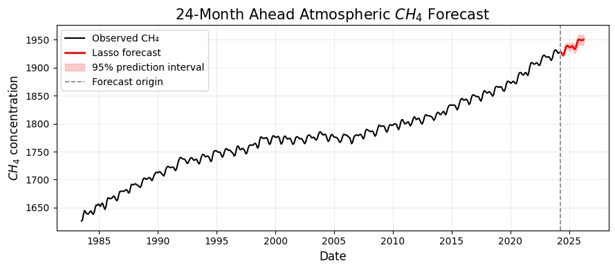
Figure 4: Atmospheric CH4 time series showing the historical observations and the selected model forecasts across the unseen holdout period.
As shown in Figure 4 the forecast broadly reproduces both the longer-term movement and the recurring seasonal fluctuations observed throughout in the historical atmospheric methane series. The ability of the forecast to reproduce this behaviour is important. Because it means that the engineered feature set forecast contain sufficient information for the model to preserve the dominant structure of the series even when forecasting progressively further into the future.
The detailed forecasting behaviour becomes clearer when the holdout period is examined separately. The first experiment therefore considers the more demanding case in which no newly observed methane concentrations are supplied to the model after the forecasting process begins.
8.1 Twenty-Four-Month Recursive Forecasting
In the recursive forecasting experiment, the model is fitted using information available up to April 2024 and then forecasts the following 24 months sequentially. The first forecast is generated using historical observations. However, once the forecasting horizon extends beyond the available observations, some of the historical values required to construct lagged and rolling features no longer exist as observed data. The model must then use its own earlier predictions when constructing the information required for later forecasts.
Thus, by the later stages of the 24-month horizon, the prediction depends partly on several earlier forecasts. This makes recursive forecasting more difficult than repeatedly predicting a single month ahead because small errors can propagate through the features used for subsequent predictions.
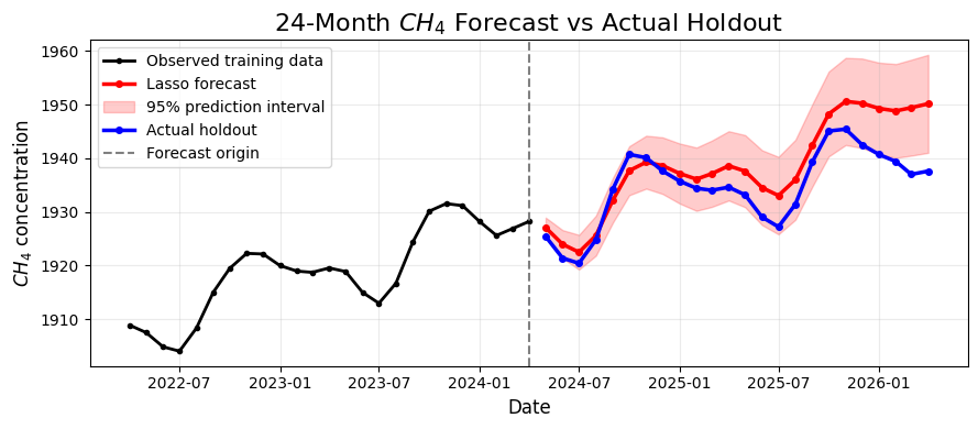
Figure 5: 24-month recursive Lasso forecast of atmospheric CH4 compared with the unseen holdout observations. Earlier predictions are used when constructing the features required for later forecasts.
As shown in Figure 5, the recursive forecast preserves the main structure of the unseen methane series. The predicted trajectory rises and falls through the seasonal cycle rather than following a simple monotonic trend, while also maintaining the broader upward movement present in the historical record.
This provides useful evidence that the selected features contain information about more than the immediate concentration level. The combination of lagged concentrations, historical changes, seasonal differences, rolling statistics, and cyclical calendar variables allows the model to retain the dominant temporal structure even when it must increasingly depend on its own previous forecasts.
A notable feature of Figure 5 is the progressive widening of the 95% prediction interval. This is expected in a multi-step recursive forecasting problem. As the horizon increases, uncertainty from earlier predictions can influence the information used to generate later forecasts. The widening interval therefore reflects the increasing uncertainty associated with forecasting further into the future without access to the observations that occur between the initial forecast origin and the later forecast dates.
8.2 Rolling One-Step-Ahead Forecasting
The second experiment evaluates the selected model using a rolling one-step-ahead forecasting framework. In this approach, a forecast is generated for each month using only the information that would have been available at that time. Once the actual methane concentration for that month becomes known, it is incorporated into the historical information used to forecast the following month.
For example, the forecast for June 2024 can use the actual observation from May 2024 because that value would already have become observable before the June forecast is made. Unlike the recursive forecast, errors are not repeatedly carried forward through the entire forecasting horizon. Each new observed concentration updates the information available to the model before the next prediction is generated.
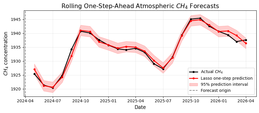
Figure 6: Rolling one-step-ahead Lasso forecasts of atmospheric CH4 across the 24-month unseen holdout period.
As seen in Figure 6, the rolling one-step-ahead forecasts follow the observed methane concentrations remarkably closely throughout the holdout period. The model captures the major rise during late 2024, the subsequent seasonal decline, the increase during late 2025, and the movement through early 2026. The resulting performance is exceptionally strong. Across the 24-month holdout period, the model achieves a mean absolute error of approximately 0.717 ppb and an RMSE of approximately 0.962 ppb. These errors are very small relative to atmospheric methane concentrations of approximately 1,900 ppb.
This shows that the selected model generalizes extremely well to observations that were not used during model development. The holdout error is also slightly lower than the average cross-validation error. While this cannot necessarily be interpreted as evidence that the holdout period was inherently easier to forecast, it provides additional support for the conclusion that the model has learned persistent temporal relationships rather than simply reproducing the training data.
The prediction intervals in Figure 6 are also substantially narrower than those in the recursive forecast shown in Figure 5. This difference follows directly from the forecasting design. Each prediction is only one month ahead, and the next forecast benefits from the newly observed atmospheric methane concentration.
8.3 Why Is the Forecasting Performance So Strong?
The agreement between the forecasts and the unseen observations is remarkably strong. Real-world forecasting problems do not always produce this level of predictive accuracy, particularly over an evaluation period spanning two years. A plausible explanation lies not only in the selected model but also in the nature of the published atmospheric methane series being forecasted.
The dataset used in this analysis is a processed observational product rather than a direct stream of unprocessed sensor measurements. The atmospheric observations collected through the monitoring network at NOAA undergo quality control and processing before the final globally averaged monthly series is produced. The resulting series is therefore cleaner and contains less short-term measurement noise.
The atmospheric methane series also contains several characteristics that are particularly favourable for forecasting. It has strong temporal persistence, a pronounced recurring seasonal structure, and relatively smooth month-to-month behaviour. These properties mean that recent observations contain substantial information about what is likely to happen in the near future.
Additionally, the feature-engineering strategy developed in this analysis was specifically designed to exploit this structure. Lagged concentrations describe the recent atmospheric level, historical differences provide information about short-term movement, seasonal differences and calendar variables represent recurring annual behaviour, while rolling statistics and trend features summarize the recent local structure of the series. The remarkably good forecasting performance is therefore best understood as the result of the combination of a carefully processed and strongly structured atmospheric time series with a feature-engineering strategy designed to represent its dominant temporal behaviour.
9. Conclusion
This analysis demonstrated how a univariate atmospheric time series can be transformed into a supervised machine-learning forecasting problem. Although no external explanatory variables were supplied to the models, substantial predictive information was extracted from the historical behaviour of the atmospheric CH4 series itself.
An important lesson from this analysis is that successful time-series forecasting depends not only on the machine-learning algorithm used but also on understanding the underlying data and designing informative historical features. The results also demonstrate that greater model complexity does not necessarily produce better forecasts. In this case, relatively simple regularized linear models achieved strong generalisation when combined with appropriate carefully engineered features.
Finally, the forecasting performance should be interpreted in the context of the data itself. The published NOAA monthly methane series represents a carefully processed large-scale atmospheric signal with strong persistence and recurring seasonal structure. These properties make the dominant behaviour of the series more predictable than many noisier real-world forecasting problems.
The complete implementation including code, detailed outputs, model tuning results, figures, and additional technical discussion are provided in the accompanying Jupyter Notebook, allowing the full forecasting workflow to be examined and reproduced.