Linear algebra is one of the most widely used branches of mathematics in science, engineering, and artificial intelligence (AI); yet it is often taught in a way that feels abstract and disconnected from real-world application. Most introductory courses in linear algebra stop at definitions and some hand-solved exercises. As a result, many students walk away knowing how to compute a determinant or eigenvalue but not knowing why these ideas matter or where they are used in real-world applications.
“After a linear algebra course most students know the terminologies; yet if you ask them how these translate into real-world they have little to no idea.”
In reality, linear algebra is everywhere. It powers modern technologies such as deep learning, computer graphics, robotics, computer vision, signal processing, financial modelling, and even the way our phones processes images. Of course, this is just a fraction of what you can do with linear algebra; there are many other applications.
This blog is the first in a three-part series designed to bridge the gap between linear algebra's mathematical theory and its real-world applications. In the first two parts (starting with this one), we will build a solid foundation by introducing the essential terminology, notation, and core ideas that form the language of linear algebra. Then, in Part III we will explore how these concepts appear in practice through a real-world example. If you are already comfortable with the fundamental concepts and prefer to explore applications, feel free to skip ahead to Part III.
The discussion presented in this blog series will omit the usual “theorem and proof” approach of many undergraduate linear algebra textbooks. The intention is to get the reader up to scratch in some of the essential ideas and notation that will be found in the more advanced linear algebra textbooks and applied research papers.
Why Learn Linear Algebra?
Linear algebra is one of the three main mathematical “languages” of AI (alongside calculus and probability). It provides a framework for representing and manipulating data efficiently. In fact, modern computers are designed to perform millions of matrix operations every second, making linear algebra one of the foundations of scientific computing.
Many popular Python libraries—including NumPy, SciPy, Pandas, TensorFlow, and PyTorch—are built almost entirely around vector and matrix operations. Even the simplest machine learning model, linear regression, relies heavily on linear algebra. This means understanding linear algebra is essential, especially if you want to thrive in the modern technological age.
GPUs are built to execute highly optimized linear-algebra operations at massive scale. Much of the deep learning's explosive growth we have seen recently stems from the inherently parallel structure of its core algorithms, which map efficiently onto commodity GPU hardware.
Linear Algebra Building Blocks
1. Scalars
A scalar is simply a single numerical value. Each element (numbers in a matrix or vector) is a scalar. Think of a scalar as a single measurement, such as: Temperature = 24°C or Salary = \$6,600.
2. Vectors
A vector is an ordered collection of numbers. Vectors are commonly written as either row vectors (horizontal) or column vectors (vertical). For example, suppose a shop sells 15 laptops, 22 phones, and 10 tablets. These sales can be represented by the column vector: \[ \mathbf{s} = \begin{bmatrix} 15 \\ 22 \\ 10 \end{bmatrix} \]
3. Matrices
Put simply, a matrix is an array of numbers organised into rows and columns. Matrices provide a convenient way to organise and store data; in fact, many real-world datasets can naturally be represented as matrices. For example, suppose we record the daily closing prices of two stocks over three consecutive days. This information can be organised into a \(2 \times 3\) matrix, where the two rows represent the stocks and the three columns represent the days: \[ P = \begin{bmatrix} p_{1,1} & p_{1,2} & p_{1,3} \\ p_{2,1} & p_{2,2} & p_{2,3} \end{bmatrix} \]
Matrices are widely used to represent pixels in images, spreadsheets, databases, neural network weights, etc. Matrices can either be square (\(n \times n\)) or rectangular (\(m \times n\)).
4. Tensors
A tensor is a generalisation of a scalar, vector, and matrix to higher dimensions. Scalars are 0th-order tensors, vectors are 1st-order tensors, and matrices are 2nd-order tensors. Higher-order tensors are particularly useful for representing data with three or more dimensions. For example, a colour image can be represented as a third-order tensor with dimensions \((\text{height} \times \text{width} \times \text{RGB channels})\). The elements of a third-order tensor are typically written as \(a_{i,j,k}\), while the elements of a fourth-order tensor are written as \(a_{i,j,k,l}\), and so on. Modern machine learning frameworks, such as TensorFlow, are named after tensors because tensors are the primary data structures used to store and manipulate data during computation.
Matrix Addition/Subtraction
Two matrices can only be added or subtracted if they have the same dimensions, which means they have the same number of rows and columns. The operation is performed element by element. For example;
Matrix subtraction works in exactly the same way, except corresponding elements are subtracted instead of added.
Note: In standard matrix algebra, a scalar cannot be directly added to a matrix because it violates the fundamental requirement that matrices must be of the same dimension. However, programming languages such as MATLAB, R, and Python allow this operation through a mechanism called broadcasting. Broadcasting temporarily expands the scalar into a matrix of identical dimensions behind the scenes, allowing element-wise addition. So, same dimension requirement is not technically violated!
- Commutative (Means; the order does not matter): \[ A + B = B + A. \]
- Associative (the grouping does not matter): \[ A + (B + C) = (A + B) + C. \]
Matrix Multiplication
Matrix multiplication is one of the most important operations in linear algebra. It combines the rows of one matrix with the columns of another. Unlike matrix addition, the two matrices do not have to be the same shape. However, the number of columns of the first matrix has to equal the number of rows of the second matrix. For example; if \(A\) is an \(n \times m\) matrix and \(B\) is an \(m \times p\) matrix, then the product \(AB\) is defined and has dimensions \(n \times p\):
\[ (n \times m)(m \times p) = n \times p. \]Notice that the number of columns in A \(= \) number of rows in B; which is (\(m \)). Each element is obtained by multiplying a row of \(A\) by a column of \(B\):
\[ AB_{ij}=\sum_{k}A_{ik}B_{kj}. \]For example,
Here, each entry of the result is the dot product of a row of the first matrix and a column of the second. For larger matrices the process is exactly the same, but repeated for every entry of the output matrix. Modern software performs these calculations efficiently for matrices with millions of elements.
- A matrix can be multiplied by a scalar, which simply multiplies every element by that number.
- Matrix multiplication is not commutative; in general, \[ AB \ne BA. \]
- Matrix multiplication is associative (the grouping does not matter): \[ A(BC)=(AB)C. \]
- Matrix multiplication is distributive over addition: \[ A(B+C)=AB+AC. \]
Matrix Transpose
The transpose of a matrix is obtained by swapping its rows and columns, i.e. the rows become columns. If \[ A = \begin{bmatrix} a_{11} & a_{12} \\ a_{21} & a_{22} \end{bmatrix}, \] then its transpose is \[ A^{T} = \begin{bmatrix} a_{11} & a_{21} \\ a_{12} & a_{22} \end{bmatrix} \]
So, why do we need it? Suppose a supermarket records sales of three products over four days. Rows represent products, columns represent days. Now imagine you want to compare sales across days instead of products. Rather than rewriting the entire dataset, we simply transpose it. The transpose allows us to switch perspectives without changing the underlying information.
Linear Systems and Solutions
A linear equation is an equation in which each variable has a power of one and the graph of the equation is a straight line/plane. A system of linear equations is a collection of one or more linear equations involving the same variables. A solution to the system is a list of numbers that makes every equation true when substituted into the variables.
A linear system can have no solution, exactly one unique solution, or infinitely many solutions. A system is called consistent if it has one or infinitely many solutions, and inconsistent if it has no solution.
Example 1: A Unique Solution
Consider the system:
\[ \begin{aligned} y &= 2x+1\\ y &= -x+4 \end{aligned} \]One way to solve this system is by graphing the two lines. The solution is the point where they intersect. Since the equations are linearly independent, they have a unique solution \((1,3)\).
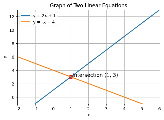
Figure 1: Two independent equations intersecting at a single point.
Example 2: Infinitely Many Solutions
Now consider the system:
\[ \begin{aligned} x+y&=2\\ 2x+2y&=4 \end{aligned} \]The second equation is simply twice the first, so it does not provide any new information. The two equations therefore are linearly dependent. When plotted they represent the same line and every point on the line satisfies both equations, so the system has infinitely many solutions.
Example 3: No Solution
Finally, consider the system:
\[ \begin{aligned} y &= 2x+1\\ y &= -x+4\\ y &= 3x-2 \end{aligned} \]The three equations are all different, so each contributes new information. However, there is no single point where all three lines intersect simultaneously. Although each pair of lines intersects, there is no point that satisfies all three equations, meaning the system has no solution.
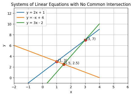
Figure 2: Three lines with no common point of intersection.
Another common example of a system with no solution is two parallel lines. Since parallel lines have the same slope but different intercepts, they never intersect. Their equations therefore contradict one another, so their system is inconsistent and has no solution.
When a system has two variables, each equation represents a line, and the solution is their point of intersection. With three variables, each equation represents a plane in 3-dimensional space, and the solution is the point where all three planes intersect. While these geometric interpretations are very helpful, they quickly become impossible to visualize in higher dimensions. Fortunately, software such as R and Python can solve these larger systems efficiently.
Matrix Notation for Linear Systems
The essential information of a linear system can be written compactly using matrices. Consider the system:
\[ \begin{aligned} x + y + z &= 6\\ 2x - y + z &= 3\\ x + 2y - z &= 3 \end{aligned} \]This can be expressed in matrix form as \(A\mathbf{x} = \mathbf{b}\), where:
The matrix \(A\) is called the coefficient matrix (or matrix of coefficients) of the system. If we append the constants from the right-hand side, we obtain the augmented matrix of the system:
\[ \left[ \begin{array}{ccc|c} 1 & 1 & 1 & 6\\ 2 & -1 & 1 & 3\\ 1 & 2 & -1 & 3 \end{array} \right] \]If a variable is missing in an equation, its coefficient is simply written as zero. This matrix notation will be important later in Part II when discussing matrix inversion.
Matrix Rank
Matrix rank is a key concept in linear algebra and it plays an important role in statistics and machine learning. It is particularly useful when solving systems of linear equations. The rank of a matrix is the number of linearly independent rows (or columns) it contains. A row is linearly independent if it cannot be written as a linear combination of the other rows. Intuitively, rank measures how much unique information is present in the system. Dependent equations do not add any new information and therefore do not increase the rank.
Consider the system of equations we had above in Example 1; Because the equations are linearly independent, the coefficient matrix has rank 2. In Example 2; The equations are linearly dependent, so the coefficient matrix has rank 1. As for Example 3; the coefficient matrix has rank 2, which is the maximum possible for a system with two unknowns. However, the augmented matrix has rank 3, meaning the system is inconsistent.
- The rank of a matrix can never exceed the smaller of its number of rows and columns.
- Full-rank matrices contain no redundant rows or columns.
- A square matrix is invertible if and only if it has full rank.
- A unique solution occurs when the coefficient matrix has full column rank and the system is consistent.
- If the coefficient matrix and augmented matrix have the same rank, the system is consistent. If the augmented matrix has a larger rank, the system has no solution.
Conclusion
In this Part I, we have introduced the foundational building blocks of linear algebra—scalars, vectors, matrices, and tensors—and explored how they interact through operations such as addition, multiplication, and transposition. We also examined how linear systems can be expressed compactly using matrix notation, and how concepts like matrix rank help us understand whether a system has solutions.
In Part II, we will build on this foundation by exploring more advanced concepts such as determinants, matrix inverses, eigenvalues, eigenvectors, and the powerful Singular Value Decomposition (SVD).